back to main 210A page
Week 1
Agresti and Finlay:
1.3, 1.8-1.10, 1.16
2.2-2.3, 2.6, 2.13, 2.16, 2.20-2.21, 2.27-2.28, 2.30, 2.34-2.35
Week 2
Agresti and Finlay:
3.3-3.4, 3.9-3.15, 3.31-3.32, 3.36-3.37, 3.45-3.46
Lab assignment
Open the file National Longitudinal Survey of Young Women 88 (sysuse nlsw88.dta) in Stata and create a log file. Use either the "*" command or a highlighter / colored ink to mark up the log file and draw attention to the salient information. It's OK if you make a few mistakes in the syntax before you get it right.
For those of you doing the non-Stata version of the course (or who are doing Stata but need a hint), here's the log.
Note that graphs won't go in the log file so you'll need to go to print them and/or go to the file menu and choose the "save graph" command. If you're not using Stata you can use the tables in the log files to make a graph in Excel or just hand sketch it (regular paper is OK).
- What kind of variable is married?
- What kind of variables are age and wage?
- For age and wage identify the range, mean, median, and inter-quartile range.
- Create a frequency table ("tab var1") for age. What is the mode?
- Create a frequency table ("tab var1 var2") for age and married.
- Create a histogram for age. Identify the mode, median, and mean. (If using stata, try the "data are discrete" option and as continuous with 5 "bins" or 3 "bins").
- Create a boxplot for age. Identify the inter-quartile range and median.
- Create a boxplot for age by married. In general, are married or single women older? Which has the lower median? 75th percentile? 25th percentile?
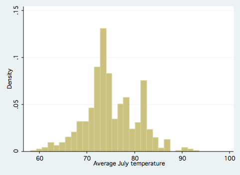
- Switch over to the weather data (sysuse citytemp.dta, clear). What are the mean, median, and inter-quartile range for july temperature?
- Create a histogram for july temperature (or use mine).
- On the weather graph, draw and label vertical lines at the mean, +/- one standard deviation, and +/- two standard deviations. About what percentage of these cities have weather within a standard deviation of the mean? What about within two standard deviations?
Week 2 and a half (relevant to week 2 thursday lecture but due with the week 3 homework)
Agresti and Finlay:
4.6 (note that "mean of the distribution" is equivalent to expected value)
Lab assignment
Imagine that a particular airport cop is so incredibly talented at detecting terrorists such that he has a probability of .999 of meeting a terrorist and realizing he's a danger but a probability of only .001 of meeting an innocent person and mistaking him for a terrorist. Further assume that one out of every ten million air passengers is a terrorist. If this cop suspects someone, what is the probability that the suspect is actually a terrorist? Please not only calculate the answer but use a tree diagram to help you. It's OK to round off "1-10^-7" as simply "1."
After a long series of wrongful arrest complaints, the cop is reassigned to a notorious border crossing where one in twenty cars is smuggling drugs and other contraband. Assume that the cop is just as good at spotting contraband as at spotting terrorists. If the cop flags down a car, what is the probability that he'll actually find contraband when he searches it?
Who would have a better track record of catching the guilty and not hassling the innocent: a talented cop on a terrorism detail or a thoroughly incompetent cop on the smuggling detail? Why? (No calculation is necessary for this last comparison).
Week 3
Agresti and Finlay: 4.8, 4.15, 4.20, 4.22, 4.29, 4.32
Lab assignment
Download a text editor and play with it. See the resources page for some links. Try opening this Stata do-file in the text editor and seeing if you get syntax highlighting. If it works, you should see the commands in one color and the quoted text in another. Try typing more commands and breaking the quotes and see what happens.
[Optional] Copy this text into an empty screen in the text editor and do a regular expression search to get it first name first:
DiMaggio, Paul
Meyer, John
Powell, Woody
Zucker, Lynne
Open a word processor and copy this text into it:
Some Boring Article
by Some Guy

Abstract
150 words of blah blah blah

Introduction
There is a growing literature on some tedious subject, all of which I will summarize for you.
Set the title, author, abstract heading, and introduction heading as the "heading 1" style. Set the abstract content and introduction content as the "normal" style. Change the heading style to be a really garish font.
Week 4
Open the file National Longitudinal Survey of Young Women 88 (sysuse nlsw88.dta) in Stata and create a log file. Use either the "*" command or a highlighter / colored ink to mark up the log file and draw attention to the salient information. It's OK if you make a few mistakes in the syntax before you get it right.
Answer the following:
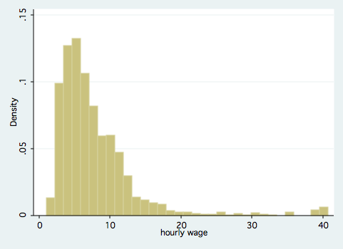
- What is the distribution of wage? (i.e., is it count, normal, right-skewed, or left-skewed). You can use my graph.
- Hand calculate the standard error of wage using the usual definition of standard error.
- Use the "regress" command (without independent variables) to let Stata find the standard error of wage. Do this three times and compare the outcomes.
- Find the bootstrapped standard error of wage (using "regress") with 10 repetitions. Do this three times and compare the outcomes.
- Find the bootstrapped standard error of wage with 1000 repetitions. Do this three times and compare the outcomes.
- Explain why one of these techniques gives identical results each times, another has only tiny variations, and another has fairly large variations.
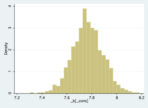
Bootstrap the regression of wage with 1000 repetitions using the "saving" option to write the results of each iteration to disk. Open the saved dataset and answer the following:
- Manually identify the bootstrapped standard error.
- Graph the bootstrapped distribution and describe the shape (or use my graph). Is the distribution of bootstrapped estimates similar to the underlying distribution of the data itself? Why?
- What does standard error (bootstrapped or otherwise) mean anyway and why is it interesting?
For those of you doing the non-Stata version of the course (or who are doing Stata but need a hint), here's the log.
Week 5
Agresti and Finlay: 5.4-5.6, 5.11, 5.14, 5.19, 5.25, 5.36-5.37, 5.40
Week 6
Agresti and Finlay: 6.3, 6.8, 6.11, 6.13, 6.19, 6.24, 6.26-27, 6.32-33
Use the NLSW 88 for the following questions. As usual, create your own log file or use mine.
- Is the mean wage statistically greater than zero? How about greater than 7.5?
- Is wage statistically different from 7 bucks?
- If you are using Stata, try doing all of this using both the regress command and by hand-calculating from the codebook information
- Is proportion married statistically different from .7 ?
- What about just among the first twenty women in the dataset ?
Week 7
Agresti and Finlay: 7.3-7.5, 7.10, 7.16-7.18
Use the NLSW 88 for the following questions. As usual, create your own log file or use mine.
- Are married women different ages than unmarried women?
- Are married women older than unmarried women?
- Do college grads make the same wages as non-college grads?
- Do Southerners make the same wages as non-Southerners?
- (Optional) Do Southern college-grads make the same wage as all other women? as Southern non-college grads?
Optional programming exercises. Use the 1978 cars data for the following questions. Here's my do-file if you get stuck and need a hint.
- Create a loop that prints the numbers 5 to 15.
- List all the return macros one gets from the command "sum weight, detail"
- Use the return macros to print to screen ("list") all the cars that are above mean + sigma for weight.
- Create a global for "withforeign", then create an "if" loop that does a codebook for all cars if the global is "1", else domestic only.
- Write a program called "listmake" that takes as its argument a part of the make, then lists all cars with that as part of its make. E.g. "listmake Toyota", "listmake toyota", and "listmake toyo" should all return the three Toyota models in the dataset.
Hint: this will require the use of both "program" and the functions "lower" and either "strpos" or "regexm"
Week 8
Agresti and Finlay: 8.5-8.7, 8.20-8.22
Use two of my datasets, one on the Dixie Chicks and another on Oscar nominations. As usual, create your own log file or use mine.
- Load my dataset on Oscar nominations for acting performances from 1948-1969 ("use http://www.sscnet.ucla.edu/08F/soc210a-1/oscars.dta, clear"). Was there an association between gender and being nominated for an Oscar? Can you guess why?
- Was there an association between the actor getting nominated and the type of screenwriter? Should an Oscar hungry actor choose to work with: a nobody, a writer with a prior writing nomination working under his own name, or a prior-nominated writer working under a pseudonym to circumvent the blacklist?
- Load my dataset on which country music radio stations blacklisted the Dixie Chicks in March of 2003 ("use http://www.sscnet.ucla.edu/08F/soc210a-1/dixie.dta, clear"). Was there was an association between who owned a radio station and whether it joined the blacklist?
- Use either the tabchi package or excel/calculator to show the Pearson residuals for each cell. Which companies were especially likely to join the blacklist?
- Calculate the odds ratio of a Clear Channel station vs a Cumulus station blacklisting the Dixie Chicks.
Weeks 9 and 10
No homework
Optional Exercises
1. Do-file, log file, graph1, graph2 or zip archive of everything